Building a GPU autoscaler that works: queueing theory and utilization metrics combined

GPU utilization was at 100% and we were scaling. Charts moving up and to the right — exactly what we wanted to see. But something felt off.

The metric wasn’t wrong. The GPUs were genuinely running at 100%. The problem is that GPU utilization is only part of the story when it comes to modern inference systems. Microbatching, KV-cache reuse, network saturation, and changing workload mixes all have complex effects on the amount of work actually getting done at “100%.” Just because your GPUs are busy doesn’t mean you’re anywhere close to the ceiling.

So we took a step back and remembered the hard lessons we’ve learned over the years and asked the real question: do new requests actually arrive faster than we can finish them?

Why utilization alone is the wrong signal

Modern inference has layers of complexity that utilization can’t see through.

Microbatching lets a single GPU process multiple requests simultaneously. When batch sizes shift — shorter prompts, more concurrent users — throughput changes dramatically while the utilization number stays pinned at 100%. KV-cache hits mean some requests complete in milliseconds with virtually no compute, again with no effect on the utilization reading. Network saturation between distributed GPU nodes can throttle effective throughput while each GPU reports full utilization.

Utilization is also a lagging indicator. It rises only after jobs have been dispatched and are actively running. By the time it peaks, the queue has already built up — and if you’re running agents, your users need snappy responses now, not several minutes from now.

The signal you actually want is upstream of all of this: how much work is arriving, and how long does each job take? Everything else follows from those two numbers.

The two shapes of inference demand

Before getting into the formulas, it helps to distinguish two types of demand that live on the same platform but have different capacity requirements.

Interactive workloads — voice agents, chat completions — arrive in Poisson bursts. They’re latency-sensitive: a user waiting for a response notices even a brief queue delay. Capacity decisions need to account for variance, not just mean throughput.

Batch workloads — video generation, bulk image jobs — are sustained and tolerant. A queue building for a few minutes is acceptable; clearing the backlog efficiently is the goal.

Same platform, different models. The capacity estimator handles both.

Little’s Law: the steady-state estimate

The core formula is Little’s Law, a result from queueing theory that holds for any stable system: the average number of items in the system equals the arrival rate times the average time each item spends there.

For GPU workers:

# Capacity estimator — simplified
arrival_rate    = queue.metrics.arrival_rate    # jobs/sec (moving average)
processing_time = avg(worker.avg for worker in active_workers)

L = arrival_rate × processing_time              # Little's Law: workers needed

If 2 jobs arrive per second and each takes 10 seconds, you need 20 concurrent workers to process them in steady state. No guessing, no sampling, no proxy metrics — just two observable quantities multiplied together.

Both inputs are continuously updated from observed behavior. Each active worker reports its average job duration back to the scheduler. These averages capture more than just processing speed — they adapt transparently to changing workload mixes, situational optimizations like KV-cache hits, and model loading conditions. When any of these shift, the per-worker averages drift accordingly and the capacity estimate corrects on the next cycle, with no manual tuning required.

Square-root staffing for interactive workloads

Little’s Law gives you the mean capacity required. Interactive workloads have variance — Poisson arrivals produce bursts where you’ll briefly see 2× or 3× the average arrival rate.

The standard result from Erlang C analysis is square-root staffing: to hold queue wait time below a target percentile, you need capacity equal to L plus a headroom term that scales with √L:

# Square-root staffing floor
beta     = 1.5                                  # service-level parameter
capacity = L + beta × sqrt(L)

For L=20 workers with β=1.5: target = 20 + 1.5×√20 ≈ 27 workers. That 35% headroom is what keeps “usually fast” from becoming “sometimes lags.” The minimum is a floor, not a ceiling — if demand drops, the estimate drops with it.

The intuition: the variance of a Poisson process scales with √λ, so the excess capacity you need to absorb bursts also scales with √L. Linear headroom (e.g., always provision 50% extra) over-provisions at low load and under-provisions at high load. Square-root staffing scales correctly in both directions.

Queue drain: recovering from a batch backlog

So just combine Little’s Law and square-root staffing and done? Not quite.

Both formulas match steady-state throughput but don’t clear an existing backlog any faster. If 100 jobs accumulated while the system was provisioning, they’ll drain at the steady-state rate — which could take a long time.

The drain term adds extra capacity specifically to clear the backlog within a target window:

# Drain formula
excess = max(0, pending_jobs - L)               # backlog above steady-state
drain  = (excess × processing_time) / drain_target_seconds

capacity = L + drain                            # batch capacity

excess is the pending count above what the steady-state workers will handle — subtracting L avoids double-counting those jobs. If 100 jobs are pending, L=5, processing time is 10s, and the drain target is 300s:

excess = max(0, 100 - 5) = 95
drain  = (95 × 10) / 300 ≈ 3.2 extra workers

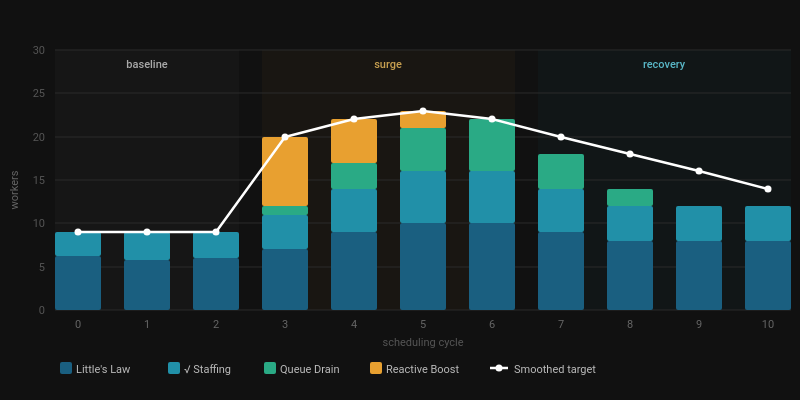
Three additive components, each independently observable: steady-state (L), backlog drain, and any reactive boost (below). Together they form the full capacity estimate for the cycle.

Reactive boost: when the model is wrong

In the end, every model is only an approximation. The three models above get us through roughly 80% of a day, but sometimes an unexpected surge arrives, someone runs a load test, or you suddenly lose connectivity to 20% of your GPU fleet.

Rejection bursts are the primary reactive signal. Square-root staffing captures most burst traffic, but when demand exceeds even that buffer, the queue starts rejecting jobs. Any burst in rejections triggers an automatic scale-up, regardless of what the predictive models say. We don’t try to model the rejection rate — a burst is evidence of saturation, and the right response is to act immediately.

Per-worker queuing is the second reactive signal. Microbatch sizes aren’t always predictable. When we observe a queue building on a specific worker — jobs waiting behind an unexpectedly long batch — we remove that worker from the dispatch rotation until its backlog clears. This trades some overall system utilization for lower per-request latency, which is the right tradeoff for interactive workloads.

Per-worker averages provide a slower continuous correction. Each active worker reports its actual job processing time. These averages naturally absorb any source of duration change — model loading, longer sequences, workload mix shifts, or lower-level engine optimizations — and the capacity estimate corrects on the next cycle without any intervention.

The combination: predictive signals handle smooth demand; reactive signals catch the exceptions.

Asymmetric smoothing: scale up fast, scale down carefully

The last piece is how the scheduler applies the estimate over time. Naive smoothing — averaging over N cycles — makes scale-up slow. That’s the wrong tradeoff for inference workloads: a demand spike should trigger provisioning immediately.

The smoothing is asymmetric:

• Scale-up is instant. When the capacity estimate rises, the new target takes effect immediately.
• Scale-down happens at a lower rate. If demand drops and recovers quickly, no instances have been terminated.

The asymmetry reflects the actual cost structure. A new GPU worker takes anywhere from one to thirty minutes to become available, depending on spare capacity, infrastructure state, and regional provider. Holding a warm instance idle costs almost nothing relative to the latency penalty of under-provisioning when demand returns.

# Asymmetric smoothing
prev    = smoothed_target[config]
target  = estimate >= prev
          ? estimate                             # scale up: instant
          : max(estimate, prev - step)           # scale down: gradual

The practical effect: brief traffic dips don’t cause terminations. If demand recovers before the gradual ramp-down completes, capacity is already there. If demand stays low long enough, the fleet scales down to match.

Putting it together

The full capacity estimate per model config, per scheduling cycle:

L        = arrival_rate × avg_processing_time   # Little's Law
drain    = (max(0, pending - L) × W) / 300      # backlog drain (5-min target)
boost    = f(rejection_burst)                   # reactive signal
raw      = L + drain + boost
smoothed = max(raw, prev_smoothed - step)       # asymmetric smoothing
target   = max(smoothed, 1)                     # floor at 1 if any demand

Each term is observable. Utilization only informs the estimates — it’s one input among many, not the signal that drives decisions.

There are still many more optimizations to explore, especially within the lower-level inference engine. But this captures the high level: a scheduler that measures what actually matters, reacts when the models fall short, and scales conservatively in the direction that’s cheap to reverse.

This way, it’s smooth sailing for the agents running on top of the infrastructure, auto-scaling seamlessly and keeping your requests flowing smoothly all day long.